2. Run an election
In this notebook, I will explain how to run a single-winner election on a voting profile with embedded voters.
[1]:
import numpy as np
import embedded_voting as ev
import matplotlib.pyplot as plt

np.random.seed(42)
Creating the profile
Let’s say we have 5 candidates and 3 groups of voters:
- The red group contains 50% of the voters, and the average scores of candidates given by this group are \([0.9,0.3,0.5,0.2,0.2]\).
- The green group contains 25% of the voters, and the average scores of candidates given by this group are \([0.2,0.6,0.5,0.5,0.8]\).
- The blue group contains 25% of the voters, and the average scores of candidates given by this group are \([0.2,0.6,0.5,0.8,0.5]\).
[2]:
scores_matrix = np.array([[.9, .3, .5, .3, .2], [.2, .6, .5, .5, .8], [.2, .6, .5, .8, .5]])
proba = [.5, .25, .25]

n_voters = 100
n_dimensions, n_candidates = np.array(scores_matrix).shape
embeddingsGen = ev.EmbeddingsGeneratorPolarized(n_voters, n_dimensions, proba)
ratingsGen = ev.RatingsFromEmbeddingsCorrelated(0.8,  scores_matrix, n_dimensions, n_candidates)

embeddings = embeddingsGen(polarisation=0.4)
profile = ratingsGen(embeddings)
We can visualize this profile, as explained in the previous notebook:
[3]:
fig = plt.figure(figsize=(15,7.5))
embeddings.plot("3D", fig=fig, plot_position=[1,2,1], show=False)
embeddings.plot("ternary", fig=fig, plot_position=[1,2,2], show=False)
plt.show()
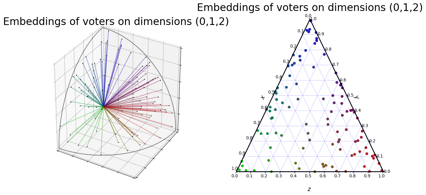
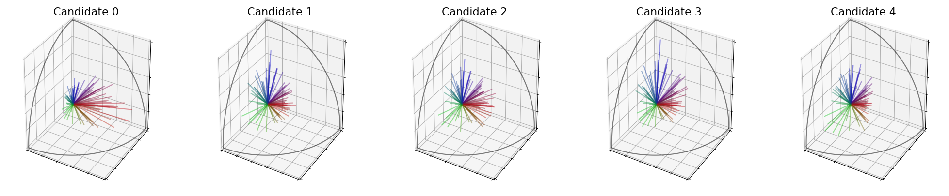
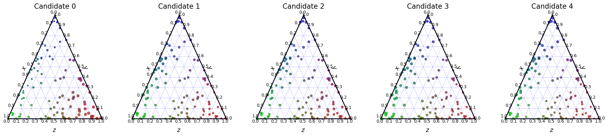
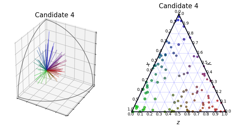
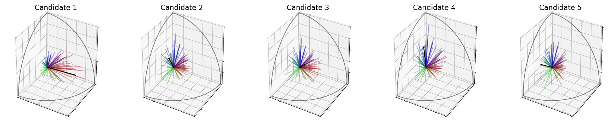
We can also visualize the candidates. Each voter is represented by a line and the length of the line represents the score the voter gives to the candidate.
[4]:
embeddings.plot_candidates(profile, "3D")
embeddings.plot_candidates(profile, "ternary")
Now, we want to determine the best candidate. Is it the Candidate 0, which is loved by the majority group? Or is it the Candidate 2, which is not hated by any group?
To decide that, we can use a whole set of voting rules. First, there is the simple rules, which are not based on the embeddings. These rules are Range voting (we take the average score) and Nash voting (we take the product of the score, or the average log score).
Notations
In the next parts of this notebook, I will use some notations:
| Notation | Meaning | Function |
|---|---|---|
| \(v_i\) | The \(i^{th}\) voter | |
| \(c_j\) | The \(j^{th}\) candidate | |
| \(s_i(c_j)\) | The score given by the voter \(v_i\) to the candidate \(c_j\) | Profile.scores[i,j] |
| \(S(c_j)\) | The score of the candidate \(c_j\) after the aggregation | ScoringRule.scores_[j] |
| \(w(c_j)\) | The welfare of the candidate \(c_j\) | ScoringRule.welfare_[j] |
| \(M\) | The embeddings matrix, such that \(M_i\) are the embeddings of \(v_i\) | Profile.embeddings |
| \(M(c_j)\) | The candidate matrix, such that \(M(c_j)_i = s_i(c_j)\times M_i\) | Profile.scored_embeddings(j) |
| \(s^*(c_j)\) | The vector of score of one candidate, such that \(s^*(c_j)_i = s_i(c_j)\) | Profile.scores[:,j] |
Simple rules
Average score (Range Voting)
This is the most intuitive rule when we need to aggregate the score of the different voters to establish a ranking of the candidate. We simply take the sum of every vote given to this candidate:
We create the election in the following cell.
[5]:
election = ev.RuleSumRatings()
We then run the election like this
[6]:
election(profile, embeddings)
[6]:
<embedded_voting.rules.singlewinner_rules.rule_sum_ratings.RuleSumRatings at 0x1e2e5614710>
Then, we can compute the score of every candidate, the ranking, and of course the winner of the election:
[7]:
print('Scores : ', election.scores_)
print('Ranking : ', election.ranking_)
print('Winner : ', election.winner_)
Scores :  [45.77999664207862, 48.88823373691184, 49.96870542210909, 52.26932370998465, 47.86098615045205]
Ranking :  [3, 2, 1, 4, 0]
Winner :  3
We can also compute the welfare of each candidate, where the welfare is defined as:
[8]:
print('Welfare : ', election.welfare_)
Welfare : [0.0, 0.4789767971790928, 0.6454766012251681, 1.0, 0.3206787832694216]
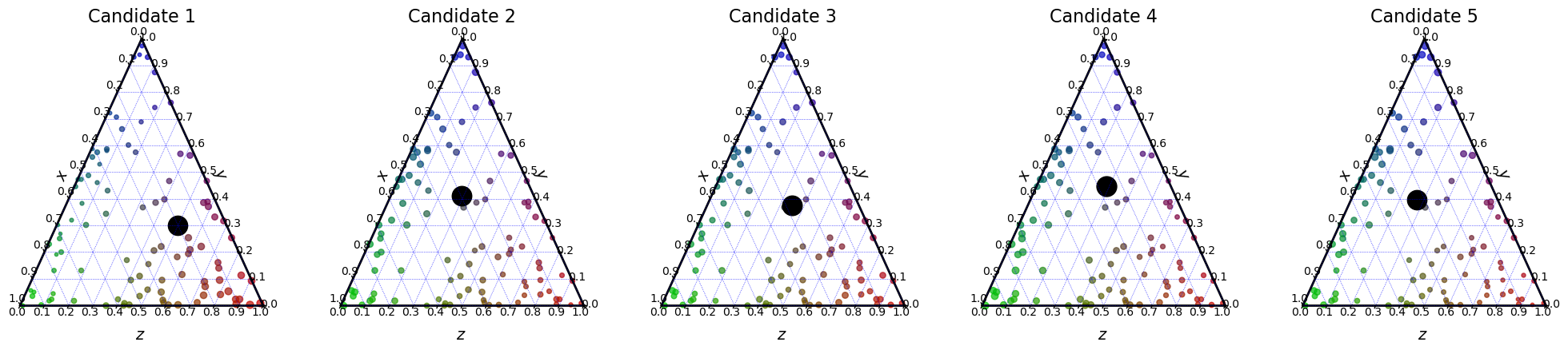
We can plot the winner of the election using the function plot_winner().
[9]:
fig = plt.figure(figsize=(10,5))
election.plot_winner("3D", fig=fig, plot_position=[1,2,1], show=False)
election.plot_winner("ternary", fig=fig, plot_position=[1,2,2], show=False)
plt.show()
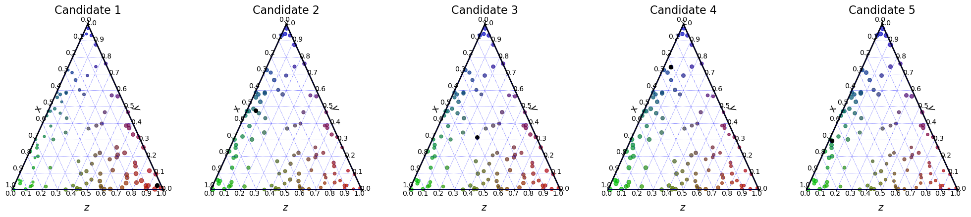
We can plot the ranking of the election using the function plot_ranking().
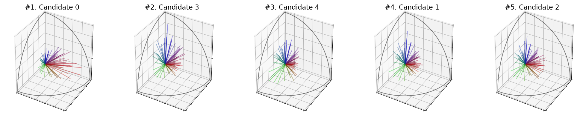
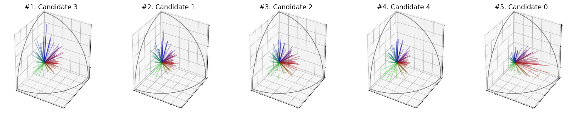
[10]:
election.plot_ranking("3D")
election.plot_ranking("ternary")

Product of scores (Nash)
The second intuitive rule is the product of the scores, also called Nash welfare. It is equivalent to the sum of the log of the scores.
We have
[12]:
election = ev.RuleShiftProduct()
election(profile, embeddings)
print('Scores : ', election.scores_)
print('Ranking : ', election.ranking_)
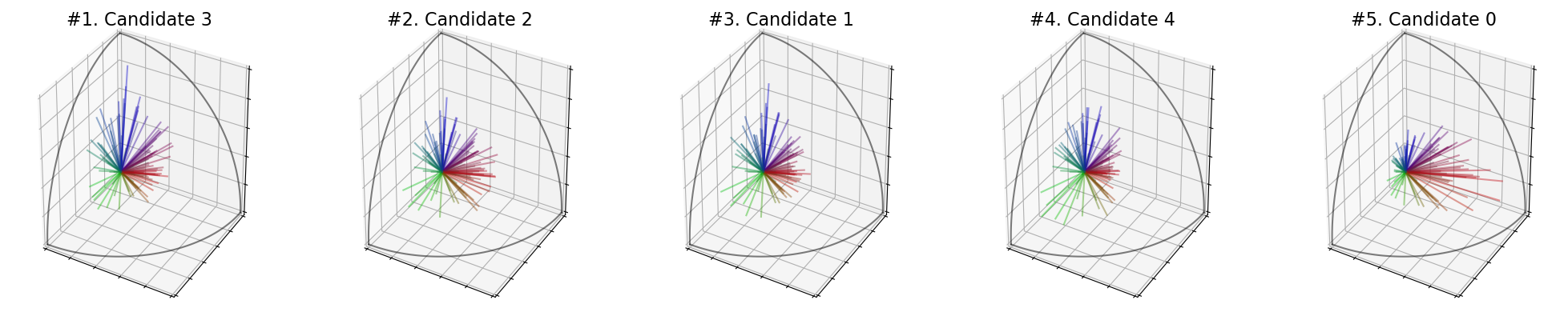
print('Winner : ', election.winner_)
election.plot_ranking("3D")
Scores :  [8.951032542639148e+38, 3.715630226275884e+39, 5.989493011777882e+39, 1.3845840911371833e+40, 2.3053960275427698e+39]
Ranking :  [3, 2, 1, 4, 0]
Winner :  3

You probably noticed that scores are composed of two elements (e.g (100, 5.393919173647501e-37)). In this particular case, the first element is the number of non-zero individual scores and the second one is the product of the non-zero scores. Indeed, if some voter gives a score of \(0\) to every candidate, the product of scores will be \(0\) for every candidate and we cannot establish a ranking.
We use similar ideas for some of the rules that will come later.
In these cases, if we have \(S(c_j) = \left ( S(c_j)_1 , S(c_j)_2 \right )\), the score used in the welfare is :
In other word, the welfare is \(> 0\) if and only if the first component of the score is at the maximum.
[13]:
print("Welfare : ",election.welfare_)
Welfare : [0.0, 0.2177889049017948, 0.3933667635308749, 1.0, 0.1088967138875542]
Geometrical rules
All the rules that I will describe now are using the embeddings of the voters. Some of them are purely geometrical, other are more algebraic. Let’s start with the geometrical ones.
All of the rules presented here do not depend on the basis used for the embeddings. Indeed, the result will not change if you change the vector basis of the embeddings (for instance, by doing a rotation)
Zonotope
The zonotope of a set of vectors \(V = \{\vec{v_1}, \ldots, \vec{v_n}\}\) is the geometrical object defined as \(\mathcal{Z}(V) = \{ \sum_i t_i \vec{v_i} | \forall i, t_i \in [0,1] \}\).
For a matrix \(M\), we have \(\mathcal Z (M) = \mathcal Z (\{ M_1, \ldots, M_n \})\).
The following figure illustrate the zonotope in 2D for a set of \(3\) vectors.
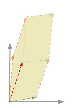
In the case of an election, the score of the candidate \(c_j\) is defined as the volume of the Zonotope defined by the rows of the matrix \(M(c_j)\) :
There is a simple formula to compute this volume, but it is exponential in the number of dimensions.
[14]:
election = ev.RuleZonotope()
election(profile, embeddings)
print('Scores : ', election.scores_)
print('Ranking : ', election.ranking_)
print('Winner : ', election.winner_)
print('Welfare : ', election.welfare_)
election.plot_ranking("3D")
Scores :  [(3, 2512.3852946433435), (3, 3478.5303669376613), (3, 3724.291234894805), (3, 4197.7832046975145), (3, 3317.721702753313)]
Ranking :  [3, 2, 1, 4, 0]
Winner :  3
Welfare :  [0.0, 0.5732444940929495, 0.7190622066290026, 1.0, 0.47783161667981705]

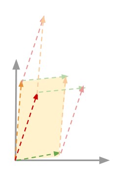
Maximum Parallelepiped
The maxcube rule is also very geometrical. It computes the maximum volume spanned by a linearly independent subset of rows of the matrix \(M(c_j)\).
The figure below shows an example of how it works.
[15]:
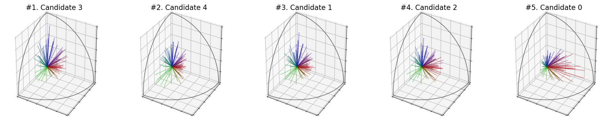
election = ev.RuleMaxParallelepiped()
election(profile, embeddings)
print('Scores : ', election.scores_)
print('Ranking : ', election.ranking_)
print('Winner : ', election.winner_)
print('Welfare : ', election.welfare_)
election.plot_ranking("3D")
Scores :  [(3, 0.1288637458094931), (3, 0.1665379237215778), (3, 0.15408795064264366), (3, 0.1825593712490694), (3, 0.15152969628703225)]
Ranking :  [3, 1, 2, 4, 0]
Winner :  3
Welfare :  [0.0, 0.701624715303474, 0.46976275304839044, 1.0, 0.42211912594341866]
SVD Based rules
Here are some of the most interesting rules you can use for embedded voters. They are based on the Singular Values Decomposition (SVD) of the matrices \(M(c_j)\).
Indeed, if we denote \((\sigma_1(c_j), \ldots, \sigma_n(c_j))\) the singular values of the matrix \(M(c_j)\), then the SVDRule() while simply apply the aggregation_rule passed as parameter to them.
Singular values are very interesting in this context because each \(\sigma_k\) represent one group of voter.
In the following cell, I use the product function, that means that we compute the score with the following formula :
[16]:
election = ev.RuleSVD(aggregation_rule=np.prod, use_rank=False, square_root=True)
election(profile, embeddings)
print('Scores : ', election.scores_)
print('Ranking : ', election.ranking_)
print('Winner : ', election.winner_)
print('Welfare : ', election.welfare_)
election.plot_ranking("3D")
Scores :  [26.741050420162296, 32.74789296371305, 33.93409961876206, 35.796076724146936, 32.132208898968436]
Ranking :  [3, 2, 1, 4, 0]
Winner :  3
Welfare :  [0.0, 0.6633710761179632, 0.7943708783523339, 1.0, 0.5953774509118517]

However, if you want to take the product of the singular values, you can directly use SVDNash(), as in the following cell.
This rule is a great rule because the score is equal to what is known as the volume of the matrix \(M(c_j)\).
Indeed, we have :
which is often described as the volume of a matrix.
[17]:
election = ev.RuleSVDNash(use_rank=False)
election(profile, embeddings)
print('Scores : ', election.scores_)
print('Ranking : ', election.ranking_)
print('Winner : ', election.winner_)
print('Welfare : ', election.welfare_)
election.plot_ranking("3D")
Scores :  [26.741050420162296, 32.74789296371305, 33.93409961876206, 35.796076724146936, 32.132208898968436]
Ranking :  [3, 2, 1, 4, 0]
Winner :  3
Welfare :  [0.0, 0.6633710761179632, 0.7943708783523339, 1.0, 0.5953774509118517]

You can take the sum of the singular values with SVDSum() :
This corresponds to a utilitarian approach of the election.
[18]:
election = ev.RuleSVDSum(use_rank=False)
election(profile, embeddings)
print('Scores : ', election.scores_)
print('Ranking : ', election.ranking_)
print('Winner : ', election.winner_)
print('Welfare : ', election.welfare_)
election.plot_ranking("3D")
Scores :  [10.281197693329844, 10.791272853780711, 10.916846435776982, 11.138673498000554, 10.697528579564]
Ranking :  [3, 2, 1, 4, 0]
Winner :  3
Welfare :  [0.0, 0.5948566218107435, 0.7413022489786075, 1.0, 0.48553076829268343]
You can take the minimum of the singular values with SVDMin() :
This corresponds to an egalitarian approach of the election.
[19]:
election = ev.RuleSVDMin(use_rank=False)
election(profile, embeddings)
print('Scores : ', election.scores_)
print('Ranking : ', election.ranking_)
print('Winner : ', election.winner_)
print('Welfare : ', election.welfare_)
election.plot_ranking("3D")
Scores :  [1.9464873750164875, 2.213040976979755, 2.1945439239678493, 2.272105557536364, 2.2490434464796065]
Ranking :  [3, 4, 1, 2, 0]
Winner :  3
Welfare :  [0.0, 0.8186078550665599, 0.7618018964165792, 1.0, 0.9291743757111914]
You can take the maximum of the singular values with SVDMax():
For single winner voting, this rule seems not very suited, because it will only maximize the satisfaction of one group. But it can be very useful for multi-winner voting (see the dedicated notebook).
[20]:
election = ev.RuleSVDMax(use_rank=False)
election(profile, embeddings)
print('Scores : ', election.scores_)
print('Ranking : ', election.ranking_)
print('Winner : ', election.winner_)
print('Welfare : ', election.welfare_)
election.plot_ranking("3D")
Scores :  [6.072281075810715, 6.186173173309101, 6.247073024447592, 6.407979709322462, 6.110288589883775]
Ranking :  [3, 2, 1, 4, 0]
Winner :  3
Welfare :  [0.0, 0.33926887430836317, 0.5206811443001008, 1.0, 0.1132191503893329]

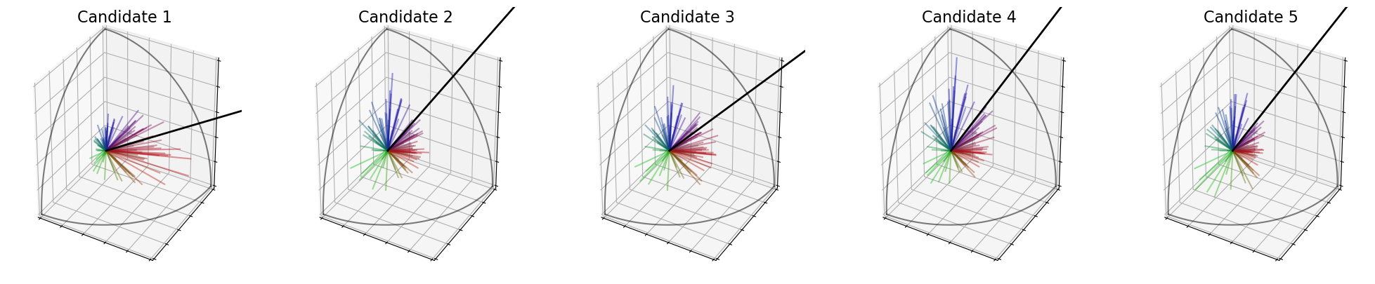
For this rule in particular, we can plot the “features” of the candidates, which actually corresponds to the position of the most important singular vector from the singular value decomposition.
[21]:
election.plot_features("3D")
election.plot_features("ternary")
Finally, there is the SVDLog() rule, which is a bit more exotic. It corresponds to the following equation :
where \(C\) is a constant passed as parameter (its default value is \(1\)).
[22]:
election = ev.RuleSVDLog(const=2, use_rank=False)
election(profile, embeddings)
print('Scores : ', election.scores_)
print('Ranking : ', election.ranking_)
print('Winner : ', election.winner_)
print('Welfare : ', election.welfare_)
election.plot_ranking("3D")
Scores :  [2.831659715452525, 2.940987770371308, 2.9627590583541927, 2.996678664966983, 2.927844515160104]
Ranking :  [3, 2, 1, 4, 0]
Winner :  3
Welfare :  [0.0, 0.6625181849748972, 0.7944502330635768, 1.0, 0.582871239882373]

The following table summarize the different rules based on the SVD :
| Name | Equation | Interpretation |
|---|---|---|
| SVDNash |
\[S(c_j) = \prod_k \sigma_k(c_j)\]
|
Nash Welfare |
| SVDSum |
\[S(c_j) = \sum_k \sigma_k(c_j)\]
|
Utilitarian |
| SVDMin |
\[S(c_j) = \min_k \sigma_k(c_j)\]
|
Egalitarian |
| SVDMax |
\[S(c_j) = \max_k \sigma_k(c_j)\]
|
Dictature of majority |
| SVDLog |
\[S(c_j) = \sum_k \text{log}\left (1+\frac{\sigma_k(c_j)}{C} \right )\]
|
Between Nash and Utilitarian |
Features based rule
The next rule is based on what is often called features in machine learning.
Indeed, it consists in solving the linear regression on \(MX_j = s^*(c_j)\) for every candidate \(c_j\). We want the vector \(X_j\) such that
It corresponds to \(X_j = (M^tM)^{-1}Ms^*(c_j)\). This is the classic feature vector for candidate \(c_j\).
In the following cell, the features of every candidate are shown in black on the 3D plots.
[23]:
election = ev.RuleFeatures()
election(profile, embeddings)
election.plot_features("3D")
election.plot_features("ternary")
Then, we define the score of candidate \(c_j\) as :
[24]:
print('Scores : ', election.scores_)
print('Ranking : ', election.ranking_)
print('Winner : ', election.winner_)
print('Welfare : ', election.welfare_)
election.plot_ranking("3D")
Scores :  [0.679363163960879, 0.596773936003501, 0.5674211903311394, 0.6579158241916001, 0.6380881542815943]
Ranking :  [0, 3, 4, 1, 2]
Winner :  0
Welfare :  [1.0, 0.2622139374587864, 0.0, 0.8084066318124928, 0.631282097850031]