7. Algorithms aggregation

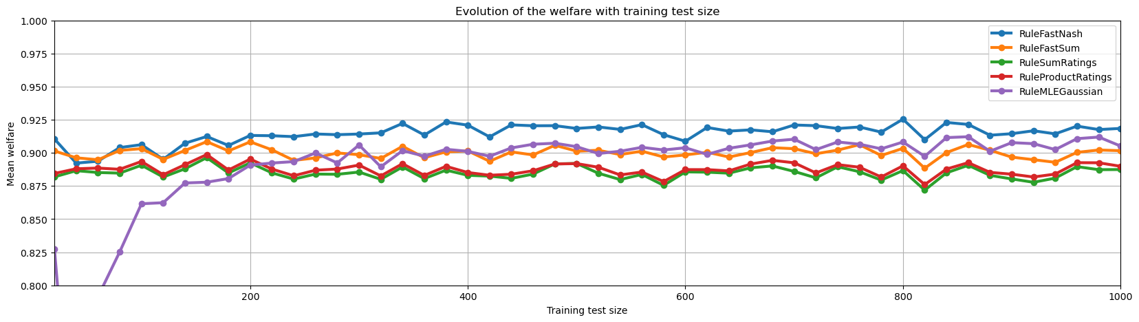
In this notebook we will compare the different voting rules on an online learning scenario. We have different aggregators with different scoring rules, and each aggregator start with 0 training data. Then each aggregator use the data from the successive aggregations to train the embeddings.

import numpy as np
import embedded_voting as ev
import matplotlib.pyplot as plt
from tqdm import tqdm
np.random.seed(42)

We will comapre 5 rules : FastNash, FastSum, SumScores, ProductScores, MLEGaussian

def create_f(A):
    def f(ratings_v, history_mean, history_std):
        return np.sqrt(np.maximum(0, A + (ratings_v - history_mean) / history_std))
    return f

list_agg = [ev.Aggregator(rule=ev.RuleFastNash(f=create_f(0)),name="RuleFastNash"),
            ev.AggregatorFastSum(),
            ev.AggregatorSumRatings(),
            ev.AggregatorProductRatings(),
            ev.AggregatorMLEGaussian()]

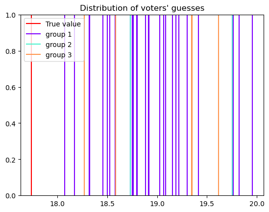
For the generator, we use a model with \(30\) algorithms in the same group \(G_1\), \(2\) algorithms in agroup \(G_2\) and \(5\) algorithms between the two (but closer to \(G_2\))

groups_sizes = [30, 2, 5]
features = [[1, 0], [0, 1], [0.3,0.7]]

generator = ev.RatingsGeneratorEpistemicGroupsMix(groups_sizes, features, group_noise=8, independent_noise=0.5)
generator.plot_ratings()

onlineLearning = ev.OnlineLearning(list_agg, generator)

Each election contains \(20\) alternatives, we run \(50\) successive elections for each experiment and run this \(1000\) times.

n_candidates = 20
n_steps = 50
n_try = 1000
onlineLearning(n_candidates, n_steps, n_try)

100%|██████████| 1000/1000 [57:38<00:00,  3.46s/it]

Finally, we can display the result of the experiment

onlineLearning.plot()