6. Multi-winner elections

We’ve already seen how to run a single-winner election with embedded voters. Now, I will explain how you can simulate multi-winner election on this framework.

I will explain in detail what you can do with the multi-winner rules IterSVD() and IterFeatures(). If you are interested and want to implement your own multi-winner rule, you can check the doc and the code for the class IterRule().

import embedded_voting as ev
import numpy as np
import matplotlib.pyplot as plt
np.random.seed(42)

Create the profile

You should start to be familiar with this part of the notebook. As always, we are creating a profile of embedded voters. This time, we have \(20\) candidates instead of \(5\), because it enables us to see what our multi-winner rules really do.

To do so, I simply use the candidates from the profile of the Notebook 2, and duplicate them 3 times. The profile is as follows :

• The red group contains 50% of the voters, and the average scores of candidates given by this group are \([0.9,0.3,0.5,0.2,0.2]\).
• The green group contains 30% of the voters, and the average scores of candidates given by this group are \([0.2,0.6,0.5,0.3,0.9]\).
• The blue group contains 20% of the voters, and the average scores of candidates given by this group are \([0.2,0.6,0.5,0.9,0.3]\).

In that way, candidates \((0, 5, 10, 15)\) are candidates of the red group, candidates \((4, 9, 14, 19)\) are candidates of the green group, candidates \((3, 8, 13, 18)\) are candidates of the blue group, and all other candidates are more “consensual”.

In the following cell, I create my profile using ParametricProfile():

scores_matrix_bloc = np.array([[.9, .3, .5, .3, .2], [.2, .6, .5, .3, .9], [.2, .6, .5, .9, .3]])
scores_matrix = np.concatenate([scores_matrix_bloc]*4, 1)

proba = [.5, .3, .2]

n_voters = 100
n_dimensions, n_candidates = np.array(scores_matrix).shape
embeddingsGen = ev.EmbeddingsGeneratorPolarized(n_voters, n_dimensions, proba)
ratingsGen = ev.RatingsFromEmbeddingsCorrelated(0.8, scores_matrix,  n_dimensions,n_candidates )

embeddings = embeddingsGen(polarisation=0.6)
profile = ratingsGen(embeddings)

The following cell displays the profile distribution:

fig = plt.figure(figsize=(15,7.5))
embeddings.plot("3D", fig=fig, plot_position=[1,2,1], show=False)
embeddings.plot("ternary", fig=fig, plot_position=[1,2,2], show=False)
plt.show()

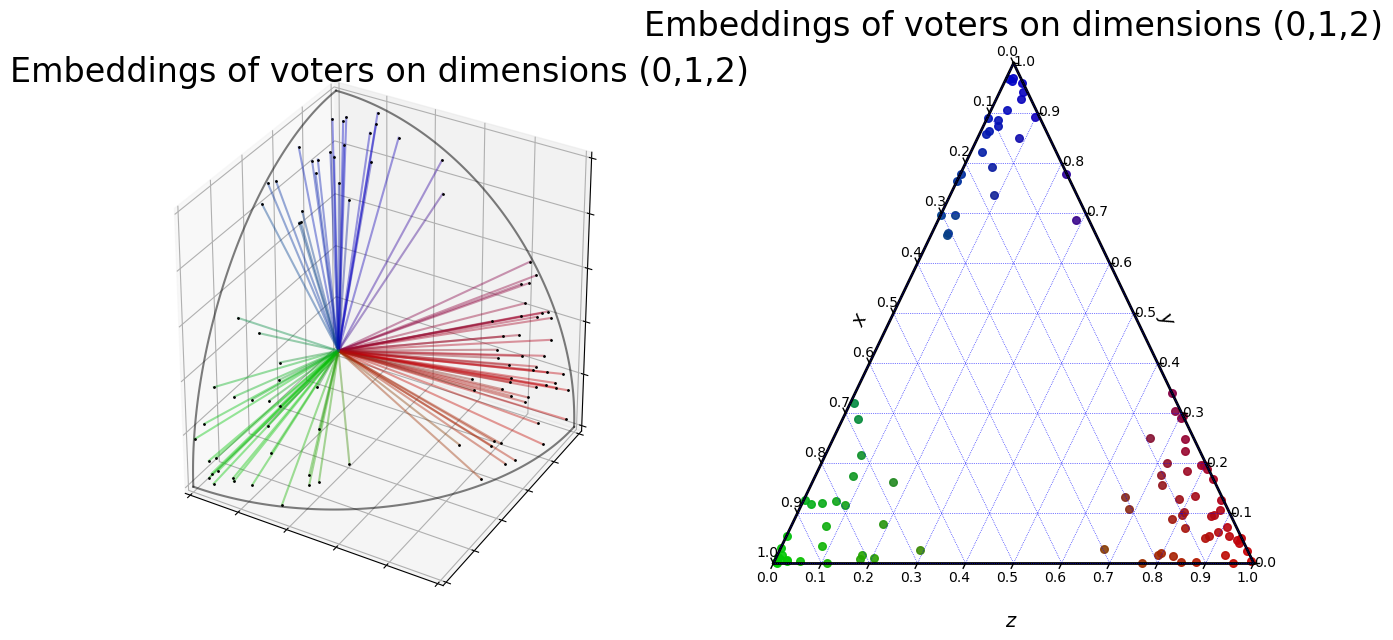
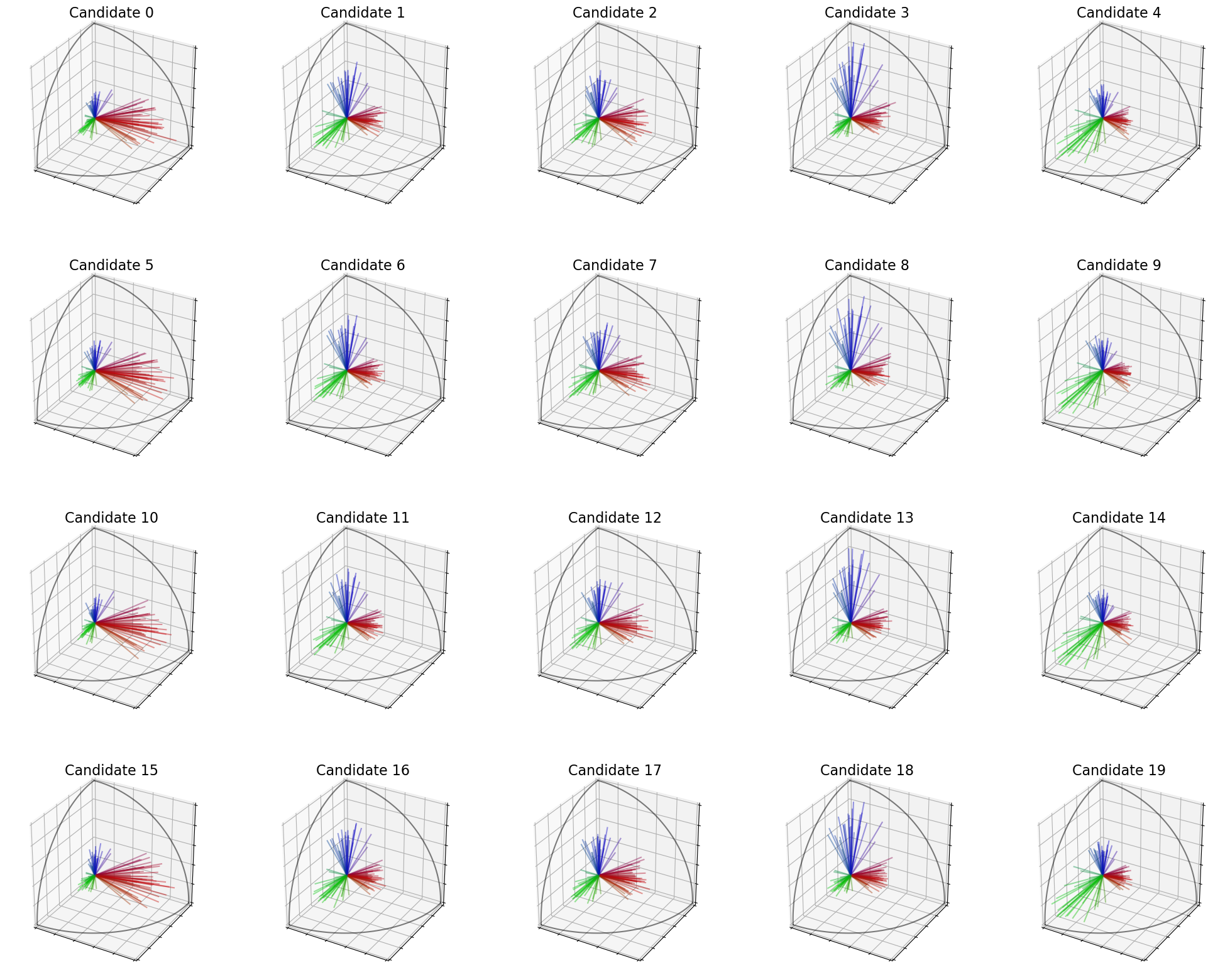
This cell displays the candidates. You can see that each column contains very similar candidates.

embeddings.plot_candidates(profile, "3D")

How IterRule work (a bit of theory)

Our goal was to elaborate rules that respects the proportionality with respect to both the scores and the embeddings of the voters. That means that if a group of voter with similar embeddings represent \(25\%\) of the population, \(25\%\) of the winning committee should be composed of their favorite candidates

To do so, we implemented an adaptation of Single Transferable Vote (STV) to profiles with embedded voters.

First, some notations :

Notations	Meaning
\(v_i\)	The \(i^{th}\) voter
\(c_j\)	The \(j^{th}\) candidate
\(s_i(c_j)\)	The score given by the voter \(v_i\) to the candidate \(c_j\)
\(M\)	The embeddings matrix, such that \(M_i\) are the embeddings of \(v_i\)
\(k\)	The size of the winning committee
\[0 \le t < k\]	The iteration number
\(w_i(t)\)	The weight of the voter \(v_i\) at time \(t\)
\(W(t)\)	The \(t^{th}\) candidate of the winning committee
\(sat_i(t)\)	The satisfaction of voter \(v_i\) with candidate \(W(t)\)

The rules we are using in this notebook are following this algorithm:

• At the initialization, the weight of all voters is equal to \(w_i(0) = 1\).

• At each step \(t \in [0, k-1[\) :

  • Apply a voting rule on the profile defined by the scores \((w_i \times s_i)\) and the embeddings matrix \(M\). The voting rule should return a score and a feature vector for each candidate. Select the candidate \(c\) not yet in the committee with the maximum score. This will be the winner \(W(t)\). Let’s denote \(v(t)\) the feature vector of this candidate.
  • We compute the satisfaction of every voter with the new candidate, which is defined as
  \[s_i(W(t)) \times \text{cos}(v(t),M_i)\]

  where \(\text{cos}\) is the cosine similarity. Therefore, a voter with embeddings close to the candidate’s features will be more satisfied than a candidate orthogonal to the features of the candidate.

  • Update the weights of the voters according to their level of satisfaction. The sum of all the removed weights should be equal to a quota of voter, for instance \(\frac{n}{k}\).

At the end, the weights of all voters should be close to \(0\).

In this notebook, I will present two rules based on this algorithm : IterSVD and IterFeatures.

• IterSVD uses a SVD based rule presented on the notebook 2 to determine the scores of the candidates. The feature vector is the vector of the SVD associated to the largest singular value. A very well-suited aggregation function to achieve proportionnality is the maximum function.
• IterFeatures is based on the Features rule presented on the notebook 2. The notion of feature vector in that case is straightforward.

Now, let’s see how it works!

Run an election

The following cell shows how you instantiate a multi-winner election.

Here we want a committee of size \(k=5\) and we are using the classic method of quota (see next section).

election = ev.MultiwinnerRuleIterSVD(k=5, quota="classic")
election(profile, embeddings)

<embedded_voting.rules.multiwinner_rules.multiwinner_rule_iter_svd.MultiwinnerRuleIterSVD at 0x20aa08c0f28>

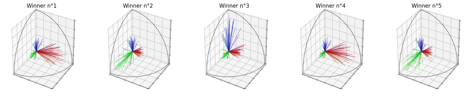
You can immediately print and plot the winning committee.

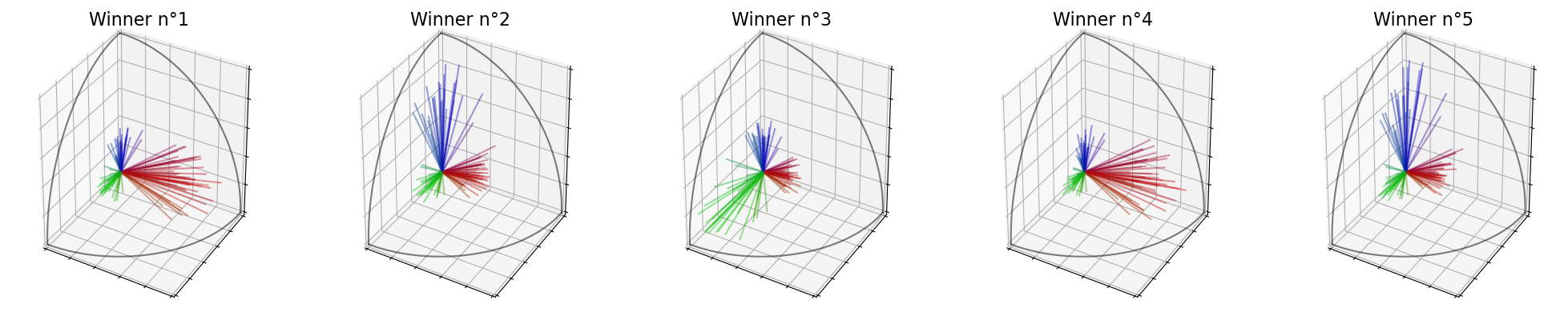
In our case, the committee contains \(3\) candidates of the red group, \(2\) candidates of the green group and \(0\) of the blue group. This gives us proportion of \((40\%, 40\%, 20\%)\) instead of the correct proportionality \((60\%, 40\%, 0\%)\).

print("Winners : ",election.winners_)
election.plot_winners()

Winners :  [5, 18, 19, 15, 3]

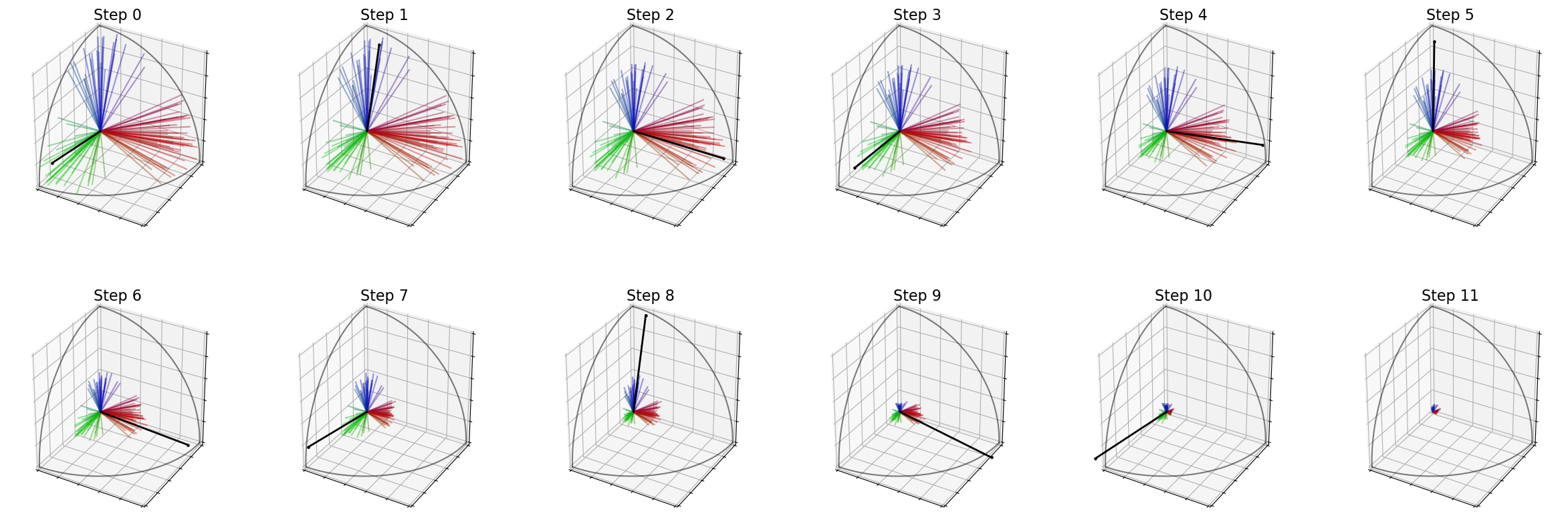
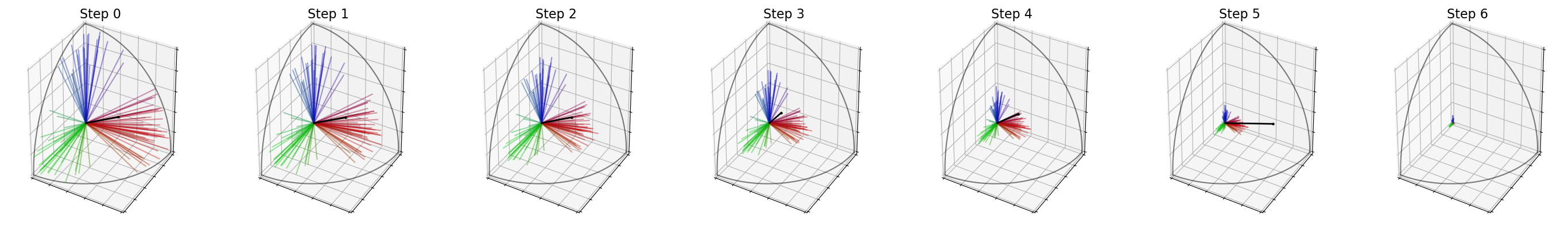
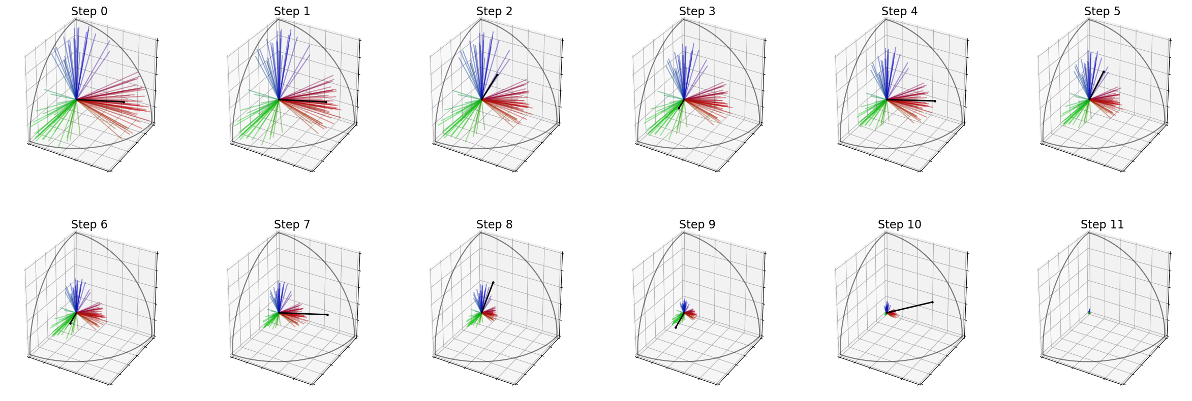
The following cell shows how to plot the evolution of the voters’ weights with time. The black vector represents the feature vector of the candidate selected at this step.

For instance, the first candidate is liked by the red group, so its vector is very similar to the vectors of voters in this group, and you can see that the weight of every voter of this group is reduced during step 2.

election.plot_weights(row_size=6)

Weight / remaining candidate :  [20.0, 20.0, 20.000000000000004, 20.000000000000004, 20.000000000000014]

Changing some parameters

You can change the method of quota using the function set_quota(). There are two possible quotas:

• Classic quota \(Q = \frac{n}{k}\).
• Droop quota \(Q = \frac{n}{k+1} + 1\).

However, there is not a big difference between the results if we use on quota or another. For instance, with \(k=5\), we obtain the same committee as before:

election.set_quota("droop")
print("Winners : ",election.winners_)
election.plot_winners()

Winners :  [5, 18, 19, 15, 3]

You can also change parameters related to the SVD, for instance the square_root parameter, which can influence the results.

Indeed, as you can see on the following cell, when we are not using the square root of the score, we give more opportunities to small groups (like the group of blue voters).

election = ev.MultiwinnerRuleIterSVD(k=5, quota="classic", square_root=False)
election(profile, embeddings)
print("Winners : ",election.winners_)
election.plot_winners()

Winners :  [5, 19, 3, 15, 14]

Changing the size of the committee

You can change the size of the winning committee, by calling the function set_k().

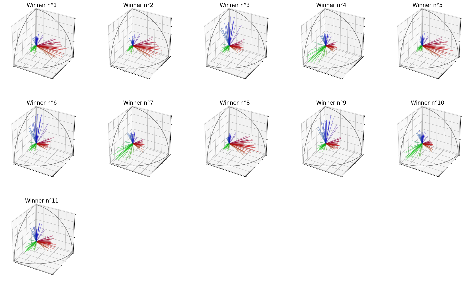
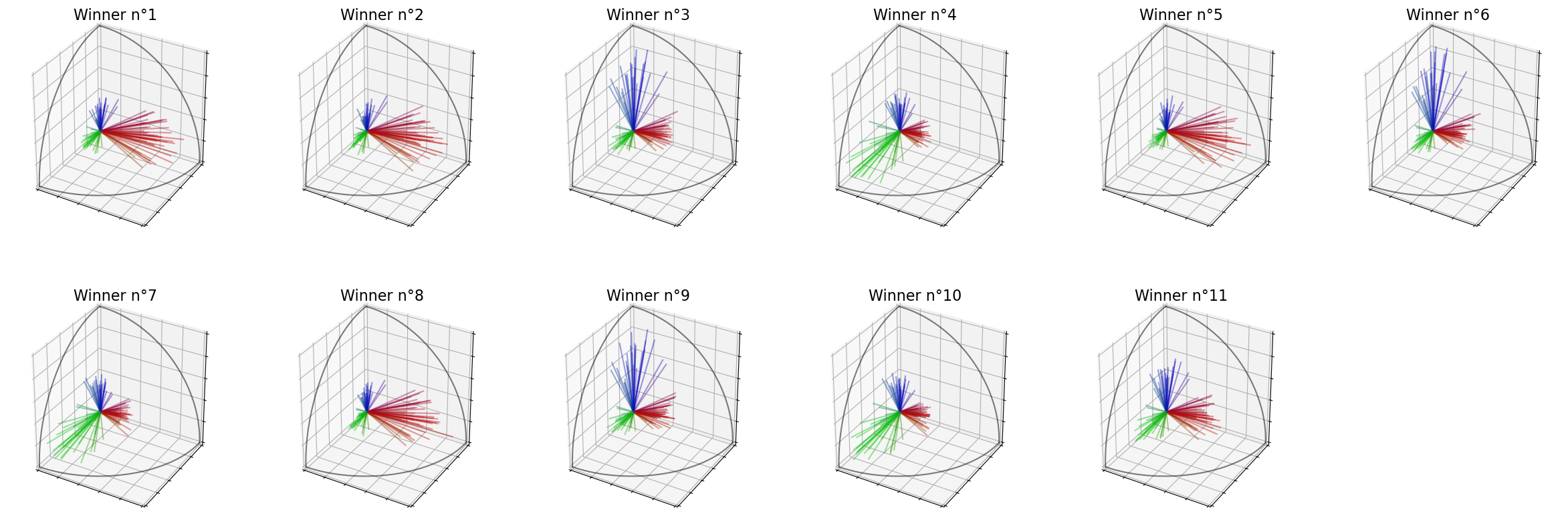
As you can see, if we set the size of the committee to \(k=11\) candidates, There are \(4\) candidates of the red group (that is the maximum possible), there are also \(4\) candidates of the green group, and \(2\) candidates of the blue group. The last candidate (actually Winner 10) is a consensual candidate.

The proportions obtained are close to the real proportions \((50\%, 30\%, 20\%)\).

election = ev.MultiwinnerRuleIterSVD()
election(profile, embeddings)
election.set_k(11)
print("Winners : ",election.winners_)
election.plot_winners()

Winners :  [5, 10, 18, 19, 15, 3, 14, 0, 8, 9, 7]

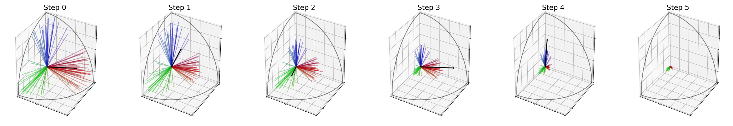
As before, we can display the evolutions of the weights of the voters, with the feature of the selected candidate at each step in black. In the end, all weights are almost \(0\).

election.plot_weights(row_size=6)

Weight / remaining candidate :  [9.090909090909092, 9.09090909090909, 9.090909090909092, 9.09090909090909, 9.090909090909092, 9.090909090909092, 9.09090909090909, 9.09090909090909, 9.090909090909088, 9.090909090909088, 9.090909090909085]

Using other SVD Rules

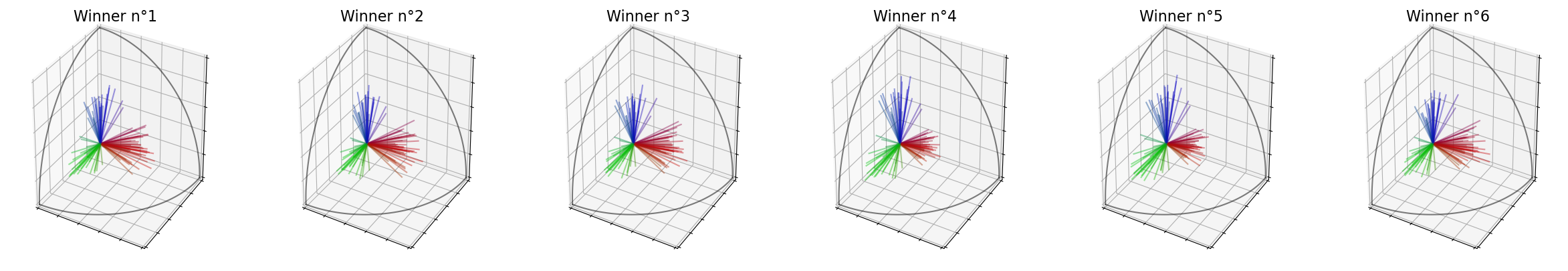
You can use another rule than the maximum for the IterSVD() function. However, the maximum is well suited for proportionality, which is not the case for other aggregation functions. For instance, with the product, we only obtain consensual candidates, as it is shown in the following cell:

election = ev.MultiwinnerRuleIterSVD(k=6, quota="classic", aggregation_rule=np.prod)
election(profile, embeddings)
print("Winners : ",election.winners_)
election.plot_winners(row_size=6)

Winners :  [7, 2, 17, 6, 1, 12]

election.plot_weights(row_size=7)

Weight / remaining candidate :  [16.666666666666668, 16.666666666666664, 16.666666666666664, 16.666666666666664, 16.666666666666664, 16.666666666666654]

IterSVD versus IterFeatures

Everything I explained earlier for IterSVD also works for IterFeatures. Let’s see how the two rules compare on some examples:

election_svd = ev.MultiwinnerRuleIterSVD(k=5)
election_features = ev.MultiwinnerRuleIterFeatures(k=5)

election_svd(profile, embeddings)
election_features(profile, embeddings)

<embedded_voting.rules.multiwinner_rules.multiwinner_rule_iter_features.MultiwinnerRuleIterFeatures at 0x20a9c67e860>

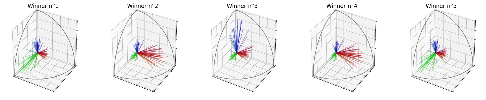
With \(k=5\), the proportions achieved by IterFeatures are \((40\%, 40\%, 20\%)\), which is more egalitarian than the \((60\%, 40\%, 0\%)\) achieved by IterSVD.

It is due to the fact that IterSVD takes into account the size of each each group to choose a winner but not IterFeatures. For the latter, the size of the group only appears when we update the weights of the voters.

print("Winners (SVD) : ",election_svd.winners_)
election_svd.plot_winners()
print("Winners (Features) : ",election_features.winners_)
election_features.plot_winners()

Winners (SVD) :  [5, 18, 19, 15, 3]

Winners (Features) :  [19, 5, 3, 10, 14]

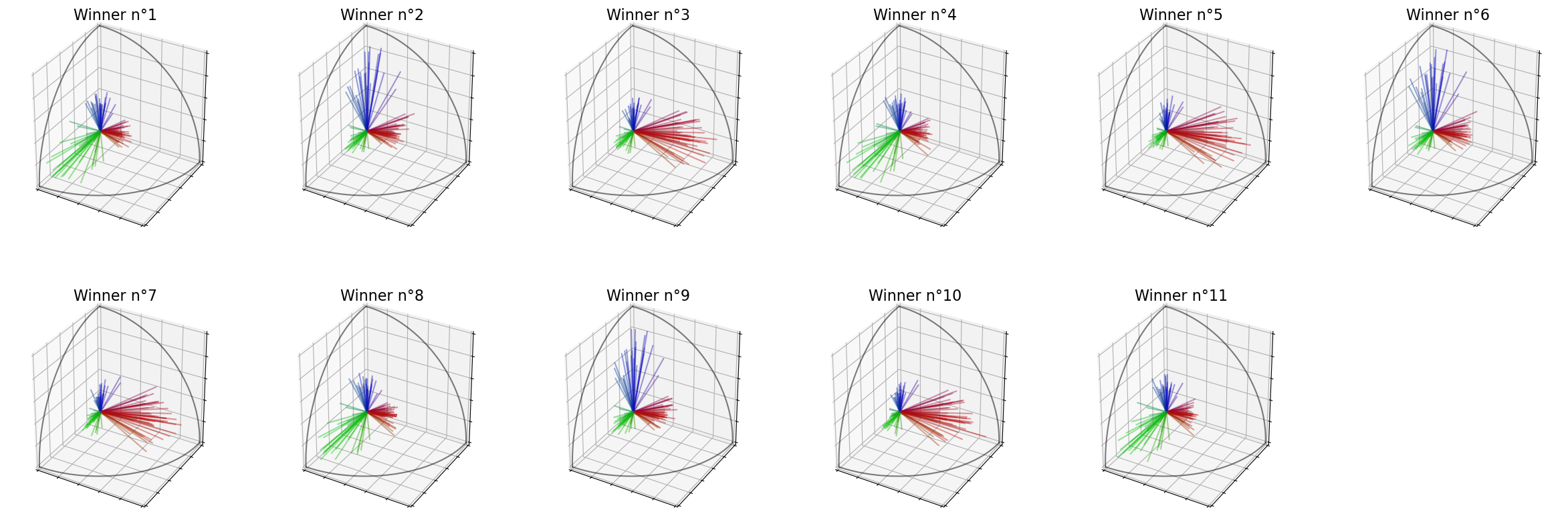
It is even clearer with \(k=11\). As you can see in the following cells, the first two candidates selected by IterFeatures are a green candidate and a blue candidate, even if the red group is the biggest.

election_svd.set_k(11)
election_features.set_k(11)

<embedded_voting.rules.multiwinner_rules.multiwinner_rule_iter_features.MultiwinnerRuleIterFeatures at 0x20a9c67e860>

print("Winners (SVD) : ",election_svd.winners_)
election_svd.plot_winners(row_size=6)
print("Winners (Features) : ",election_features.winners_)
election_features.plot_winners(row_size=6)

Winners (SVD) :  [5, 10, 18, 19, 15, 3, 14, 0, 8, 9, 7]

Winners (Features) :  [19, 3, 5, 14, 15, 18, 10, 9, 13, 0, 4]

print("IterSVD")
election_svd.plot_weights(row_size=6, verbose=False)
print("IterFeatures")
election_features.plot_weights(row_size=6, verbose=False)

IterSVD

IterFeatures