Changing Noises

This notebook investigates how the reference scenario evolves if we change: - The intensities of feature and distinct noises. - The shape of the distribution used to draw candidate utilities, feature noises, and distinct noises.

import numpy as np
import dill as pickle
import matplotlib.pyplot as plt
from tqdm import tqdm
import tikzplotlib
from multiprocess.pool import Pool

import embedded_voting as ev # Our own module

Direct load of some useful variables and functions.

from embedded_voting.experiments.aggregation import make_generator, make_aggs, f_max, f_renorm
from embedded_voting.experiments.aggregation import handles, colors, evaluate, default_order

n_tries = 10000 # Number of simulations
n_training = 1000 # Number of training samples for trained rules
n_c = 20

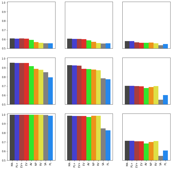
Changing Noise Intensities

Computation

res = np.zeros( (9, 3, 3) )
with Pool() as p:
    for j, distinct_noise in enumerate([.1, 1, 10]):
        for k, group_noise in enumerate([.1, 1, 10]):
            generator = make_generator(feat_noise=group_noise, dist_noise=distinct_noise)
            training = generator(n_training)
            testing = generator(n_tries*n_c).reshape(generator.n_voters, n_tries, n_c)
            truth = generator.ground_truth_.reshape(n_tries, n_c)

            list_agg = make_aggs(distinct_noise=distinct_noise, group_noise=group_noise)
            res[:, j, k] = evaluate(list_agg=list_agg, truth=truth,
                                    testing=testing, training=training, pool=p)

100%|███████████████████████████████████████████████████████████████████████████| 10000/10000 [00:19<00:00, 523.39it/s]
100%|███████████████████████████████████████████████████████████████████████████| 10000/10000 [00:17<00:00, 563.79it/s]
100%|███████████████████████████████████████████████████████████████████████████| 10000/10000 [00:15<00:00, 644.25it/s]
100%|███████████████████████████████████████████████████████████████████████████| 10000/10000 [00:15<00:00, 650.89it/s]
100%|███████████████████████████████████████████████████████████████████████████| 10000/10000 [00:15<00:00, 629.96it/s]
100%|███████████████████████████████████████████████████████████████████████████| 10000/10000 [00:15<00:00, 653.53it/s]
100%|███████████████████████████████████████████████████████████████████████████| 10000/10000 [00:15<00:00, 649.56it/s]
100%|███████████████████████████████████████████████████████████████████████████| 10000/10000 [00:16<00:00, 613.23it/s]
100%|███████████████████████████████████████████████████████████████████████████| 10000/10000 [00:15<00:00, 656.05it/s]

We save the results.

with open('noises_intensity.pkl', 'wb') as f:
    pickle.dump(res, f)

Display

fig, ax = plt.subplots(3,3, figsize=(12,12))

n_agg = len(list_agg)
for j in range(3):
    for k in range(3):
        ax[j,k].bar(np.arange(n_agg), res[:, k, 2-j], color=[colors[agg.name] for agg in list_agg], width=1)
        ax[j,k].set_ylim(0.5,1.01)
        ax[j,k].set_xlim(-1, n_agg)
        if k != 0:
            ax[j,k].get_yaxis().set_visible(False)
            ax[j,k].set_yticks([])
        if j == 2:
            ax[j,k].set_xticks(np.arange(n_agg))
            ax[j,k].set_xticklabels([handles[agg.name] for agg in list_agg], rotation=90)
        else:
            ax[j,k].get_xaxis().set_visible(False)
            ax[j,k].set_xticks([])

plt.ylabel("Average relative utility")
tikzplotlib.save("noises_intensity.tex")

# Save figure:
plt.savefig("noises_intensity.png")

# Show the graph
plt.show()

Changing Noise Distributions

Finally, we try different noise functions to deviate from a normal distribution. First we try wider and thiner distributions, using gennorm, and then we try skewed distributions, using skewnorm. In all cases, mean and standard deviations stay the same, only the higher moments are altered.

This analysis is not shown in the paper due to space constraints.

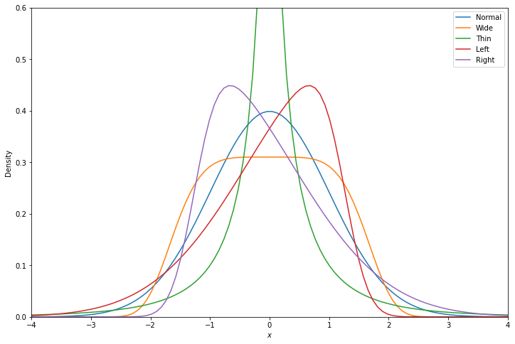
Considered Distributions

For illustration, we display the density of each considered distribution, normalized with 0 mean and unit standard deviation.

from scipy.stats import gennorm, skewnorm, norm
def normalize(rv, a, x):
    _, var = rv.stats(a, moments='mv')
    scale = 1/np.sqrt(var)
    mean, _ = rv.stats(a, scale=scale, moments='mv')
    return rv.pdf(x, a, loc=-mean, scale=scale)

plt.figure(figsize=(12, 8))
x = np.linspace(-4, 4, 100)
plt.plot(x, norm.pdf(x), label='Normal')
plt.plot(x, normalize(gennorm, 5, x), label='Wide')
plt.plot(x, normalize(gennorm, .5, x), label='Thin')
plt.plot(x, normalize(skewnorm, -5, x), label='Left')
plt.plot(x, normalize(skewnorm, 5, x), label='Right')
plt.legend()
plt.xlabel('$x$')
plt.ylabel('Density')
plt.xlim([-4, 4])
plt.ylim([0, .6])
plt.show()

Computation

def create_gennorm(beta=1):
    std = gennorm.rvs(beta, scale=1, size=100000).std()
    scale = 1/std
    def f1(size):
        return gennorm.rvs(beta, scale=scale, size=size)
    return f1


def create_skewnorm(beta=1):
    std = skewnorm.rvs(beta, scale=1, size=100000).std()
    scale = 1/std
    def f1(size):
        return skewnorm.rvs(beta, scale=scale, size=size)
    return f1

list_noise = [None, create_gennorm(5), create_gennorm(0.5), create_skewnorm(-5), create_skewnorm(5)]
dist_names = ["N", "W", "T",  "L", "R"]

res = np.zeros((9, 5))
# No need to recompute base case
with open('base_case_results.pkl', 'rb') as f:
    res[:, 0] = pickle.load(f)[:-1]
list_agg = make_aggs()

with Pool() as p:
    for i in range(1, 5):
        generator = make_generator(truth=ev.TruthGeneratorGeneral(list_noise[i]),
                                  feat_f=list_noise[i],
                                  dist_f=list_noise[i])
        training = generator(n_training)
        testing = generator(n_tries*n_c).reshape(generator.n_voters, n_tries, n_c)
        truth = generator.ground_truth_.reshape(n_tries, n_c)

        res[:, i] = evaluate(list_agg=list_agg, truth=truth,
                             testing=testing, training=training, pool=p)

100%|███████████████████████████████████████████████████████████████████████████| 10000/10000 [00:19<00:00, 505.82it/s]
100%|███████████████████████████████████████████████████████████████████████████| 10000/10000 [00:16<00:00, 624.14it/s]
100%|███████████████████████████████████████████████████████████████████████████| 10000/10000 [00:20<00:00, 478.08it/s]
100%|███████████████████████████████████████████████████████████████████████████| 10000/10000 [00:13<00:00, 756.62it/s]

We save the results.

with open('noises_function.pkl', 'wb') as f:
    pickle.dump(res, f)

Display

plt.figure(figsize=(12,5))

for i, agg in enumerate(list_agg):
    plt.bar([j-0.5+0.09*i for j in range(5)], res[i,:],  color=colors[agg.name],
            label=handles[agg.name], width=0.09)

plt.legend()
plt.xticks([i*1 for i in range(5)], dist_names)
plt.xlabel("Noise distribution")
plt.ylabel("Average relative utility")
plt.ylim(0.7,1)
plt.xlim(-0.8,4.5)

tikzplotlib.save("noise_function.tex")
# save figure:
plt.savefig("noise_function.png")
plt.show()

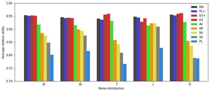
We note that MA is no longer a maximum-likelihood estimator as it assumes an incorrect underlying model. The same holds for its approximations PL and PL+. And indeed MA is no longer a de facto upper bound of performance: it is outperformed in case R, and even more in case T, by EV/EV+.